
→ →
Data Arithmetic module enables to perform arbitrary point-wise operations on a single image or on the corresponding points of several images (currently up to eight). And although it is not its primary function it can be also used as a calculator with immediate expression evaluation if a plain numerical expression is entered. The expression syntax is described in section Expressions.
The expression can contain the following variables representing values from the individual input images:
| Variable | Description |
|---|---|
d1, …, d8 |
Data value at the pixel. The value is in base physical units,
e.g. for height of 233 nm, the value of d1
is 2.33e-7.
|
m1, …, m8 | Mask value at the pixel. The mask value is either 0 (for unmasked pixels) or 1 (for masked pixels). The mask variables can be used also if no mask is present; the value is then 0 for all pixels. |
bx1, …, bx8 | Horizontal derivative at the pixel. Again, the value is in physical units. The derivative is calculated as standard symmetrical derivative, except in edge pixels where one-side derivative is taken. |
by1, …, by8 | Vertical derivative at the pixel, defined similarly to the horizontal derivative. |
x | Horizontal coordinate of the pixel (in real units). It is the same in all images due to the compatibility requirement (see below). |
y | Vertical coordinate of the pixel (in real units). It is the same in all images due to the compatibility requirement (see below). |
In addition, the constant π is available
and can be typed either as π or
pi.
All images that appear in the expression have to be compatible. This means their dimensions (both pixel and physical) have to be identical. Other images, i.e. those not actually entering the expression, are irrelevant. The result is always put into a newly created image in the current file (which may be different from the files of all operands).
Since the evaluator does not automatically infer the correct physical units of the result the units have to be explicitly specified. This can be done by two means: either by selecting an image that has the same value units as the result should have, or by choosing option Specify units and typing the units manually.
The following table lists several simple expression examples:
| Expression | Meaning |
|---|---|
-d1 | Value inversion. The result is very similar to Invert Value, except that Invert Value reflects about the mean value while here we simply change all values to negative. |
(d1 - d2)^2 | Squared difference between two images. |
d1 + m1*1e-8 | Modification of values under mask. Specifically, the value 10−8 is added to all masked pixels. |
d1*m3 + d2*(1-m3) | Combination of two images. Pixels are taken either from image 1 or 2, depending on the mask on image 3. |
In the calculator mode the expression is immediately evaluated as it is typed and the result is displayed below Expression entry. No special action is necessary to switch between image expressions and calculator: expressions containing only numeric quantities are immediately evaluated, expressions referring to images are used to calculate a new image. The preview showing the result of an operation with images is not immediately updated as you type; you can update it either by clicking or just pressing Enter in the expression entry.

→ →
It is often useful to compare the corresponding scan lines from different images – in particular trace and retrace. This can be done using Multiprofile and selecting the two images as 1 and 2 in the Images list. The selected scan line is displayed on the image. It can be moved around with mouse or the scan line number can be entered numerically using Scan line.
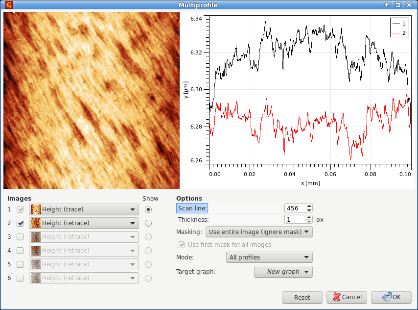
Basic usage of multiprofile module, with trace and retrace images selected as 1 and 2 and a the corresponding pair of profiles displayed in the graph.
The profiles can be read simultaneously from up to six images. Enable and disable individual images using the checkboxes next to the image number. Any of the enabled images can be displayed in the small preview, which is controlled by selecting them using Show.
Since the graph shows mutually corresponding profiles, all images must have the same pixel and physical dimensions and must also represent the same physical quantity. Image 1 is special in this regard. It cannot be unselected and it defines the dimensions and other properties. In other words, all the other images must be compatible with image 1.
Options in the lower right part include the standard thickness (averaging) control, the same as for the normal profile tool, masking options and target graph for the extracted profiles. Masks can be either taken from the corresponding images, or the mask on the first image can be used for all – if Use first mask for all images is ticked.
Instead of extracting the individual profiles, the module can also do simple statistics and plot summary curves – mean curve with lower and upper bounds. This is controlled by Mode.

→ →
Immerse insets a detailed, high-resolution image into a larger image. The image the function was run on forms the large, base image.
The detail can be positioned manually on the large image with mouse. Button can then be used to find the exact coordinates in the neighbourhood of the current position that give the maximum correlation between the detail and the large image. Or the best-match position can be searched through the whole image with .
It should be noted that correlation search is insensitive to value scales and offsets, therefore the automated matching is based solely on data features, absolute heights play no role.
Result Sampling controls the size and resolution of the result image:
- Upsample large image
- The resolution of the result is determined by the resolution of the inset detail. Therefore the large image is scaled up.
- Downsample detail
- The resolution of the result is determined by the resolution of the large image. The detail is downsampled.
Detail Leveling selects the transform of the z values of the detail:
- None
- No z value adjustment is performed.
- Mean value
- All values of the detail image are shifted by a constant to make its mean value match the mean value of the corresponding area of the large image.

→ →
Images that form parts of a larger image can be merged together with Merge. The image the function was run on corresponds to the base image, the image selected with Merge with represents the second operand. The side of the base image the second one will be attached to is controlled with Put second operand selector.
If the images match perfectly, they can be simply placed side by side with no adjustments. This behaviour is selected by option None of alignment control Align second operand.
However, usually adjustments are necessary. If the images are of the same size and aligned in direction pependicular to the merging direction the only degree of freedom is possible overlap. The Join aligment method can be used in this case. Unlike in the correlation search described below, the absolute data values are matched. This makes this option suitable for merging even very slowly varying images provided their absolute height values are well defined.
Option Correlation selects automated alignment by correlation-based search of the best match. The search is performed both in the direction parallel to the attaching side and in the perpendicular direction. If a parallel shift is present, the result is expanded to contain both images fully (with undefined data filled with a background value).
Option Boundary treatment is useful only for the latter case of imperfectly aligned images. It controls the treatment of overlapping areas in the source images:
- First operand
- Values in overlapping areas are taken from the first, base image.
- Second operand
- Values in overlapping areas are taken from the second image.
- Smooth
- A smooth transition between the first and the second image is made through the overlapping area by using a weighted average with a suitable weighting function.

→ →
Stitching is an alternative to the merge module described above. It is mainly useful when the relative positions of the image parts are known exactly because the positions entered numerically. They are initialised using image offsets, so if these are correct, the stitched image is formed automatically. Buttons for each part revert manually modified offsets to the initial ones.

→ →
Two slightly different images of the same area (for example, before and after some treatment) can be croped to intersecting area (or non-intersecting parts can be removed) with this module.
Intersecting part is determined by correlation of larger image with center area of smaller image. Images resolution (pixels per linear unit) should be equal.
The only parameter now is Select second operand - correlation between it and current image will be calculated and both images will be cropped to remove non-intersecting near-border parts.

→ →
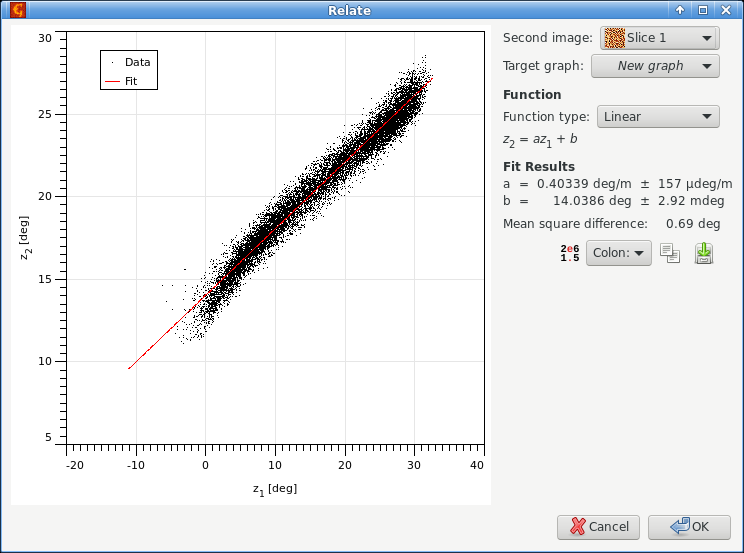
When data in two images are related in a simple manner, for instance they differ by a constant calibration factor, this function helps finding the relation.
The graph in the left part shows pixel values of the second image (selected as Second image) plotted as a function of corresponding pixel values in the current image. When a simple relation between the values exist, all the points lie on a single curve. Note that for large images only a small, randomly selected subset of pixel values is plotted in the graph.
Several simple relations can be fitted to the point data, such as proportion, offset, linear relation or quadratic relation. The fit parameters are immediately evaluated and displayed in the table below and the corresponding relation plotted. All pixel values are used for fitting, even if only a subset is displayed.
→ →
This module finds local correlations between details on two different images. As an ideal output, the shift of every pixel on the first image as seen on the second image is returned. This can be used for determining local changes on the surface while imaged twice (shifts can be for example due to some sample deformation or microscope malfunction).
For every pixel on the first operand (actual window), the module takes its neighbourhood and searches for the best correlation in the second operand within defined area. The position of the correlation maximum is used to set up the value of shift for the mentioned pixel on the first operand.
- Second operand
- Image to be used for comparison with the first operand - base image.
- Search size
- Used to set the area whera algorithm will search for the local neighbourhood (on the second operand). Should be larger than window size. Increase this size if there are big differences between the compared images.
- Window size
- Used to set the local neighbourhood size (on the first operand). Should be smaller than search size. Increasing this value can improve the module functionality, but it will surely slow down the computation.
- Output type
- Determines the output (pixel shift) format.
- Add low score threshold mask
- For some pixels (with not very pronounced neighbourhood) the correlation scores can be small everywhere, but the algorithm anyway picks some maximum value from the scores. To see these pixels and possibly remove them from any further considerations you can let the module to set mask of low-score pixel shifts that have larger probability to be not accurately determined.

→ →
This module searches for a given detail within the image base. It can produce a correlation score image or mark resulting detail position using a mask on the base image.
- Correlation kernel
- Detail image to be found on the base image. The dimensions of one pixel in both images must correspond.
- Use mask
- If the detail image has a mask you can enable this option. Only the pixels covered by the mask then influence the search. This can help with marking of details that have irregular shape.
- Output type
- There are several possibilities what to output: local correlation maxima (single points), masks of kernel size for each correlation maximum (good for presentation purposes), or simply the correlation score.
- Correlation method
- Several correlation score computation methods are available. There are two basic classes. For Correlation the score is obtained by integrating the product of the kernel and base images. For Height difference the score is obtained by integrating the squared difference between the kernel and base images (and then inverting the sign to make higher scores better). For both methods the image region compared to the kernel can be used as-is (raw), it can be levelled to the same mean value or it can be levelled to the same mean value and normalised to the same sum of squares, producing the score.
- Threshold
- Threshold for determining whether the local maximum will be treated as “detail found here”.
- Regularization
- When the base image regions are locally normalised, very flat regions can lead to random matches with the detail image and other odd results. By increasing the regularization parameter flat regions are suppressed.
Neural network processing can be used to calculate one kind of data from another even if the formula or relation between them is not explicitly known. The relation is built into the network implicitly by a process called training which employs pairs of known input and output data, usually called model and signal. In this process, the network is optimised to reproduce as well as possible the signal from model. A trained network can then be used to process model data for which the output signal is not available and obtain – usually somewhat approximately – what the signal would look like. Another possible application is the approximation of data processing methods that are exact but very time-consuming. In this case the signal is the output of the exact method and the network is trained to reproduce that.
Since training and application are two disparate steps they are present as two different functions in Gwyddion.

→ →
The main functions that control the training process are contained in tab Training:
- Model
- Model data, i.e. input for training. Multiple models can be chosen sequentially for training (with corresponding signals).
- Signal
- Signal data for training, i.e. the output the trained network should produce. The signal image must be compatible with model image, i.e. it must have the same pixel and physical dimensions.
- Training steps
- Number of training steps to perform when is pressed. Each step consists of one pass through the entire signal data. It is possible to set the number of training steps to zero; no training pass is performed then but the model is still evaluated with the network and you can observe the result.
- Starts training. This is a relatively slow process, especially if the data and/or window size are large.
- Reinitializes the neural network to an untrained state. More precisely, this means neuron weights are set to random numbers.
- Masking Mode
- It is possible to train the network only on a subset of the signal, specified by a mask on the signal data. (Masking of model would be meaningless due to the window size.)
Neural network parameters can be modified in tab Parameters. Changing either the window dimensions or the number of hidden nodes means the network is reinitialized (as if you pressed ).
- Window width
- Horizontal size of the window. The input data for the network consists of an area around the model pixel, called window. The window is centered on the pixel so, odd sizes are usually preferred.
- Window height
- Vertical size of the window.
- Hidden nodes
- Number of nodes in the “hidden” layer of the neural network. More nodes can lead to more capable network, on the other hand, it means slower training and application. Typically, this number is small compared to the number of pixels in the window.
- Power of source XY
- The power in which the model lateral dimensions units should appear in the signal. This is only used when the network is applied.
- Power of source Z
- The power in which the model “height” units should appear in the signal. This is only used when the network is applied.
- Fixed units
- Fixed units of the result. They are combined with the other units parameters so if you want result units that are independent of input units you have to set both powers to 0. This is only used when the network is applied.
Trained neural network can be saved, loaded to be retrained on different data, etc. The network list management is similar to raw file presets.
In addition to the networks in the list, there is one more unnamed network and that of the network currently in training. When you load a network the network in training becomes a copy of the loaded network. Training then does not change the named networks; to save the network after training (under existing or new name) you must explicitly use .

→ →
Application of a trained neural network is simple: just choose one from the list and press . The unnamed network currently in training is also present in the list under the label “In training”.
Since neural networks process and produce normalised data, it does not perserve proportionality well, especially if the scale of training model differs considerably from the scale of real inputs. If the output is expected to scale with input you can enable option Scale proportionally to input that scales the output with the inverse ratio of actual and training input data ranges.